GENETIC DRIFT

Genetic drift refers to random fluctuations in allele frequencies due to chance events (see figure 6.4, pg. 142). The previous lectures have all dealt with deterministic (predictable) evolutionary forces often referred to as linear pressures. Genetic drift is a stochastic (random) force that can scramble the predictable effects of selection, mutation, and gene flow. While it might seem that a random force would be of little significance to evolutionary "progress" (we'' confront this loaded term later), genetic drift is an extremely important force in evolution. However, its strength depends on the size of the population, as a simple exercise in coin tossing will illustrate. In ten tosses you might easily get seven heads; in 1000 tosses, however, you would never get 700 heads with a "fair" coin. The same sort of random fluctuation in allele frequencies can occur in small populations: consider a bag full of red and green marbles each in equal frequency; pull out a small handful and the frequency in your hand will probably not equal the frequency in the original bag. Let that handful determine the frequency in a new population that grows back to the original population size. A second small handful will randomly shift the frequency to yet another frequency. If you pulled out all the marbles in the bag (= large population) then the frequency would be maintained exactly in the next generation. Genetic drift is not a potent evolutionary force in very large randomly mating populations.

To illustrate the consequences of genetic drift we will consider what happens when drift alone is altering the frequencies of alleles among many small populations. To illustrate this we need to understand Population structure, which describes how individuals (or allele frequencies) in breeding populations vary in time and space. This structure is determined by the combined effect of deterministic and stochastic forces. We will introduce the idea of population structure by showing how genetic drift and inbreeding can change the frequencies of genotypes in populations.

Consider a grid of small populations (e.g., ponds in Minnesota), all with the same small population size and all starting at time t with p = q= 0.5. Through time each population will experience genetic drift due to random sampling and the frequencies in each population will diverge. The distribution of frequencies changes over time from a tight distribution (all 0.5), to a flat distribution (some populations at p = 0.1, some at 0.9 and all frequencies in between), to fixation (p =1.0) or loss (p = 0.0) of the alleles in all populations (see figure below). Fixation is when all alleles in the population are A; this necessarily implies loss of the a allele ("fixation" or "loss" should only be used with reference to a specific allele). If each population starts at p = 0.5, then at the end, when all populations have lost their variation, 50% of the populations will be fixed for the A allele and 50% will be fixed for the a allele (latter = "loss" for the A allele, get it?). If the initial frequency was p = 0.7, then 70% of the populations would be fixed for the A allele (again, assuming no selection, migration, mutation).

Main Points: 1) total variation does not change; variation goes from within populations (no variation between populations) to between populations (no variation within populations). 2) genetic divergence of populations entirely by chance! (no selection). This is why genetic drift can be an important force in evolution.

At the start of this drift process in our array of populations, p = 0.5 and there are 2pq = 0.5 = 50% heterozygotes. When all populations in the array have fixed or lost the allele, there can be no heterozygotes (i.e., 0%). This shows that the proportion of heterozygotes decreases as drift proceeds (this also occurs when there is inbreeding which can also be thought of as a sampling error phenomenon). We can quantify this process as follows: the proportion of heterozygotes in the "next " generation is a function of the proportion of heterozygotes in the present generation and the "rate" at which drift proceeds: Ht+1 = Ht[1 - (1/2N)] where H = the proportion of heterozygotes in the population (or in the array of populations) and N = population size. This can be extended over many generations as follows: Ht = H0[1 - (1/2N)]t where t refers to the number of generations in the future and 0 refers to the present (or starting) generation. Looking at these equations it is clear that with small population sizes, heterozygosity will be lost quickly (drift will proceed quickly), whereas in large populations there will be little loss of heterozygosity.

If we consider our grid of populations again, we note that as drift proceeds and each deme

becomes a bit different from every other deme, the variation among demes increases. Like the loss of heterozygosity due to drift, the increase in the variation among demes depends on the population size. This variation can be described as Vt = p(1-p)[1 - (1 - 1/2N)t]. Note at t=0, Vt = 0 because the term in brackets = 0. As the number of generations proceeds, the variation among populations (Vt) increases rapidly if N is small, but slowly if N is large.

A general result as drift proceeds in small populations is a deficiency of heterozygotes, and reciprocally, an excess of homozygotes. This is also a common result when there has been inbreeding (= mating between relatives). In fact genetic drift and inbreeding are related phenomena. The relation between the frequencies of expected versus observed heterozygotes allows us to determine the inbreeding coefficient, F = (He - Ho)/He (subscripts e and o mean expected and observed, respectively).

One effect of inbreeding is to increase the frequency of homozygotes (and thus, necessarily, decrease the frequency of heterozygotes). Note: while the frequency of genotypes change with inbreeding, the frequencies of alleles remains the same (assuming no selection, migration, mutation). Refer back to the data table presented on page 2 of Lecture 6 to convince yourself that those data could be a result of inbreeding: F=(0.343 - 0.14)/0.343 = 0.59. When the allele frequency is not zero, but there is a complete absence of heterozygotes , F = 1. As an exercise, work through the data in table 5.2, pg.98. Does this illustrate high or low inbreeding?

Genetic variation is generally "lost" by the action of genetic drift. This is true if we follow the fate of one deme over time. Note, however, that in our array of populations, variation is "lost" within demes, but the variation in the total system is preserved, i.e., the allele frequency in the entire metapopulation does not change, only the genotype frequencies and allele frequencies within individual demes).

Inbreeding also has the effect of increasing the variance among the individual demes of a larger population. As such, drift and inbreeding are closely related evolutionary forces. Recall that the variance = 1/N_(X-xi)2. In a random mating population with p = 0.4, f(AA) = 0.16, f(Aa) = 0.48, f(aa) = 0.36. If the alleles act in an additive manner, the heterozygotes will be intermediate and close to the mean in phenotype and will contribute little to the variance; with inbreeding most individuals are homozygous, and thus would deviate from the mean and the variance would be greater. In effect, inbreeding makes the distribution of phenotypes more "bimodal" by essentially redistributing the alleles from all three genotypes into the two homozygotes (see figure 6.5, pg. 143).

Population structure is usually quantified by a simple statistic known as Fst. This stands for the "fixation" index resulting from comparing sub populations to the total population, and is used to quantify the proportion of genetic variation that lies between subpopulations within the total population. An important way of thinking of this problem is to compare the mean heterozygosity averaged across all demes to the heterozygosity that would result if all demes were pooled into one big population. Heterozygosity is the proportion of heterozygotes in the population and is defined as H = 2 p q. Note that heterozygosity is zero at "fixation", the case where only one allele exists (p = 0 or 1), and that heterozygosity is at a maximum when alleles are equally frequent (e.g., p = q = 0.5). [For completeness, H = 1- (p2 + q2) which follows from Hardy-Weinberg above. In the case of more than two alleles, we can't just use p and q, so the following expression for heterozygosity works more generally: H = 1 - _xi2 where xi is the frequency of the "ith" allele, and summation is across all i alleles. The expression 1 - (p2 + q2) is identical to 1 - _xi2 when there are only two alleles].

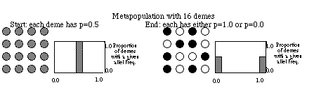
In our metapopulation example above, on the left all demes have p = 0.5 and the allele frequency for the entire array is also p = 0.5. Right away you can se that there in no differentiation among demes. To quantify this we use Fst which is calculated as Fst = (Ht - meanHs) / Ht, where Ht = 2 (pooled p) (pooled q) [note that pooled q = (1-pooled p)], and meanHs = the average of H values for each of the individual demes (i.e., 2 p q for each deme, averaged across all demes). For the left-hand metapopulation Ht = 2(0.5)(0.5) = 0.5, and meanHs = 0.5 also. Thus , Fst = (0.5 - 0.5) / 0.5 = 0.0. What does this mean? In English this says that none of the variation in this system of demes lies between demes; the population structure is zero. Since there is variation (i.e., p _ 0) all of the variation lies within demes.

Now consider the metapopulation system on the right above. The pooled allele frequency is 0.5 because half of the demes are fixed for the A allele (p = 1.0) and half are fixed for the a allele (p = 0.0). Hence the Ht value is 2 (pooled p) (pooled q) = 2(0.5)(0.5) = 0.5. The meanHs value is very different. Each deme has a heterozygosity of zero (either p or q is zero in all demes), so the average Hs value is 0.0. Hence, for the metapopulation on the right, Fst = (0.5 - 0.0) / 0.5 = 1.0. In English this means that all (100%) of the variation in the system lies between the demes. By definition then, none of the variation lies within demes, which we know because the little circles are either filled or empty. By now it should be apparent that in Fst values can range between the two extremes of zero and one that we have just illustrated. As genetic drift proceeds, Fst values will increase, but the balance between drift and "linear pressures" will determine what equilibrium Fst reaches (later lecture).

A further clarification: The "speed" or "intensity" of genetic drift is actually determined by the effective population size (Ne). This may differ from the total population size (N) if some individuals do not breed. Two examples where Ne differs from N are cases of different mating system and temporal fluctuations in population size. When the number of breeding males (Nm) _ number of breeding females (Nf), the effective population size can be quite different from the actual population size. The relation is: Ne = 4NmNf/(Nm + Nf). If Nm = Nf = N/2, then Ne = N. But if a single male does all the mating (approximated in elephant seals) then Ne = 4 (because Nf/(1+Nf) is approx. = 1). So the population genetics of elephant seals and sage grouse will be very different from that of large populations of insects.

With population bottlenecks where the population size drops to a small number in one generation, the effective population size is not just the average of N's for each generation. To estimate the Ne, one calculates the harmonic mean population size as follows:

1/Ne = 1/t_1/Nt where t = the number of generations and Nt = the population size at each generation. Thus with population sizes of 100, 100, 20, 100 the arithmetic mean = 80 but 1/Ne = 1/4(1/100 + 1/100 + 1/20 + 1/100) = 1/4(0.08) = 0.02, so Ne = 1/0.02 = 50. Thus the smaller population size has a disproportionate effect on the effective population size. This is a very important issue in conservation efforts concerning endangered species.

DRIFT AND MUTATION

Drift will tend to reduce heterozygosity (for our purposes this equals the proportion of heterozygotes), mutation will introduce new alleles which will serve to increase heterozygosity. This provides yet another example of a "fight" between opposing evolutionary forces. When the mutation rate is close to the reciprocal of the population size, heterozygostity will be high (i.e., a considerable amount of variation will exist in the population). The "balance" of this equilibrium can be described by an equation for the equilibrium frequency of heterozygotes:

H Å Plug in Ne's and u's to determine balance: when Ne = 1/u, H = 0.8; when u>1/Ne then heterozygosity will be higher; when u<1/Ne heterozygosity will be lower.

DRIFT AND GENE FLOW

Gene flow can counteract the loss of heterozygosity due to drift as well as counteract the random divergence of allele frequencies among populations. The balance between these two opposing forces can be described by an equation for the equilibrium variance among populations

V(among pops.) Å . As m increases, the variance decreases (faster homogenization); as Ne increases, the variance decreases (drift acts more slowly with larger Ne). Major conclusion is that it takes very little gene flow to keep two "populations" homogeneous, as little as one reproductive migrant between populations per generation! See figure 5.13, pg. 128.

A number of different methods have been developed to estimate migration rates from standing patterns of allele frequency variation. This rests on the fact that Fst values are a result of a "balance" between gene flow and drift. One can calculate Fst from molecular markers, and if an estimate of effective population size is available, migration can be estimated from the following relation: Fst Å 1/(4Nem + 1). By rearranging the formula and plugging in trial values you can see that low values for m result in high values for Fst, and high values of m give low values of Fst. This follows from the homogenizing effect of gene flow on allele frequency variation among populations.

The nature of population differentiation can depend on population structure. Typical scenarios include a Continent-Island model (gene flow from continent to island), an Island model (equal probability of gene flow among several/many populations), Stepping Stone model (gene flow is sequential among populations), Continuous Model (e.g., carpet of individuals). In all cases (except Island model) there can be Isolation by Distance simply reflecting incomplete homogenization of populations due to incomplete flow of genes among all populations.